Financial Derivatives

When I started to work for my current company, I have struggled to get one simple overview of this universe. Instead I had to consult many sources, lot of them were going deep into details of one particular financial product. An I was not and still I am not interested in details of investment banking but just needed simple overview.

Over the time I took notes, and kept them for myself, getting information mostly from wikipedia or investopedia. I have posted it here, just in case that it might help someone in the same position that I was.

The world of derivative products is not that complicated. From my (developer's point of view) understanding the basics of derivatives is easy. The finance guys make it bit more complicated by using special vocabulary. For instance selling and option might be called "writing an option". The price of the stock at the time that the broker and the investor exchange the option might be called "Final Reference" or "Spot Price" and so on. You might also understand a product (such as future) but you might get confused by the way it is priced – that is the way that the brokers and investors agree on prices (percentage, basis points, spreads).

• Basic vocabulary and terms
• Financial instruments
• Financial derivatives
  • Options
    • Call Option
    • Put Option
    • Delta, Implied Volatility
    • Strategies
    • Options and Hedging
    • Barrier Options
    • Warrants
    • Options pricing
  • Futures and Forwards
    • Futures and Forward pricing
    • Futures and Forward rolls
  • Convertible Bonds and Reverse Convertibles
    • Convertible Bonds
    • Reverse Convertibles
  • Swaps
    • Volatility and Variance Swaps
    • Total Return Swaps
  • ETFs
    • Net Asset Value
    • Creation Redemption
  • Other Crazy Stuff
    • Autocallables
    • Program Trading

Basic vocabulary and terms

There are two entities in this business:

• Asset Manager - a company which has collected large amount of money and invests this money hoping in regular profit. Asset Manager can be also called Buy Side, because historically and probably still he buys more, but he sells as well. So a buy side can be pension fund, mutual fund a big private equity or a hedge fund – in general anyone with enough money.
• Broker - usually a bank. It is the one that gives to Asset Managers what they need. That is the access to the shares and they also create the derivative products that the buy side can use either to risk or to hedge himself while buying some shares. Brokers are called Sell Side as well, because they sell more than buy, even though, they do both (as well as Asset Managers).

Underlying - underlying is anything that you can buy. Usually shares (stocks) or commodities but in some circumstances and underlying can be also a future. The idea is that it “underlies” the derivatives product. For instance you can buy an option on stock of Google. In that case the stock of Google is the underlying. The derivatives are products that are derived from the underlying. An option gives you the right to buy the underlying at some time in the future. A forward will oblige you to buy a stock at the price that you have agreed at some point in the future. A swap will obligate to exchange the underlying for something else. You could create an agreement to swap at some point 200 shares of Google stocks for 1000 liters of beer. This kind of swap would be a derivative with 2 underlyings (shares of google and beer).

Short - means to sell, shorting something means selling that given underlying.

Long - means to buy, being long in something means to buy and underlying and keep it.

List of financial instruments

Financial instruments are anything that you can trade on the markets. Derivatives as such as one category of financial instruments but unlike the basic once, they are "made of" them.

• Equities - stocks, shares
• Debt - bonds or mortages. This products are also called Fixed Income products, because the borrower or issuer aggree on regular payments
• FX - Currencies and Rates
• Commodities - oil, gold, whatever. Not really Financial Instrument, but you can trade it and the derivatives can be based on these as well
• Derivatives - further described in this article. Products derived from all of the other once with additional conditions and rules

Financial Derivatives

This list of financial derivatives is definitely not complete and it is just a try for some logical segregation (which can be sometimes quite hard in this field)

• Options and stratgies - Options give the right to buy or sell and are a basic building block. Two or more options in the same time form strategies, which give interesting exposures.
• Forwards and Futures - the obligation to buy something in the future for fixed price.
• Convertible Bonds - enable the change of a bond into stock
• Swaps Variance, Volatility or Return Swaps - basically exchanging performance or volatility of one stock for other stock's
• ETFs - Exchange-Traded Fund. Can be seen as a stock composed of other stocks
• Others: Autocallables, Accumulators, Program Trading and many other magic stuff

Options

There are two basic types of Options: CALL which gives the owner the right to buy and PUT giving the owner the right to sell. These two basic types can then be composed to form a "strategy". Strategy is just a fancy world used for buying or selling two options at the same time. As you can see later one can choose to do that for multiple reasons.

Call Option

Call is the right, but not the obligation to buy given underlying (stock or commodity) at given price until given date.

A trader who believes that stock's price will increase can buy the right to purchase the stock (he buys call option) at a fixed price, rather than just purchase the stock itself. He would have no obligation to buy the stock, only the right to do so until the expiration date. The price that he will pay for that option is called Premium. If the stock price at expiration (also called Spot Price) is above the agreed price (also called Strike) by more than the premium paid, he will profit i.e. if S>X, the deal is profitable. If the stock price at expiration is lower than the exercise price, he will let the call contract expire worthless, and only lose the amount of the premium. The option is less expensive than the shares itself. For less money the trader can control larger number of shares. That is why we talk about leverage.

Options parameters:

• Premium - the priced paid for the option
• Strike - the agreed price at which the underlying will be bought
• Expiry date (maturity) - the date at which the option expiries (until when you can use it)
• Settlement- either the real underlying is exchanged at expiration date ("Physical") or money is exchanged in place of the underlying ("Cash").

To visualize the options and other derivatives one can use the pay-off charts. On the X-axes of the charts we have the price of the underlying (commodity or stock) and on the Y-axes we have the total profit.

Put option

Put option gives the owner the right to sell the stock for given strike price, otherwise all other parameters are the same.

A trader who believes that a stock's price will decrease can buy the right to sell the stock at Strike price. He will be under no obligation to sell the stock, but has the right to do so until the expiration date. Logically the one who sold him the option will have buy the stock from him (if at some point the option will really get used) If the stock price at expiration is below the exercise price by more than the premium paid, he will profit. If the stock price at expiration is above the exercise price, he will let the put contract expire worthless and only lose the premium paid. Again here are the 2 pay off chats. If you bought a PUT for a MSFT stock with strike 100 for 10 dollars, you bought yourself the right to sell MSFT stock for 100 dollars. Now if the price is 90, you didn't lose anything but did not get anything either. On the other hand if the price did not move and it is still 100, you lost your 10 dollars. That shall be clear from the pay-off chart.

One has to understand, one the market one can buy or sell both types CALLs and PUTs. The outcome of each operation is different. The following chart, shows all 4 operations that can be done.

Delta and Implied Volatility

Delta always and implied volatility sometimes are parameters that the brokers provide with the price of the option, when they want to sell you one.

Delta expresses in percent the change in the price of the option with respect to change in price of the underlying. That is how much will the option price change if the underlying stock moves up or down. Delta is one of the so called Greeks that are briefly discussed later. Delta is expressed in percentage. If a stock costs 10$ and an option (with some maturity) is selled for 5 dollars and the Delta of the option is 50%, then if the stock goes to 11$, the option will go to 5.5%. That is called a delta adjustment. The broker at some point proposes a price to the investor and provides the delta as well. If the investor buys in next hour, he knows what the price of the option will be at the deal time.

Delta is always positive for a CALL and negative for a PUT. If a price of the underlying goes down, then the price you pay for the right to sell such share on some fixed price goes up. If the price of the underlying falls from 10 to 1, and you had an option giving you the right to sell for 5, you are lucky since, since you will be selling much above the market. It's clear that price of such option goes up. The reverse is true for the call. If the price of the underlying goes from 10 to 15, and you wanted to buy an option with strike 12. The broker was willing to sell you such option for 11 before, but it's price went definitely up.

Implied Volatility is another parameter sometimes provided by the brokers when giving the prices. In order to provide the price for any given option, the broker estimates the volatility of the market in the future. Implied Volatility is such estimation. Options are priced by using different variations of Black Sholes furmula. The basic idea behind this formula states, that the price of an option does depend only on it's parameters, current price of the option and the estimated volatility of the market. Of course when a broker gives a price of an option, the price will depend also on other factors, such as whether the broker has any shares of the given underlying already. But in theory, the broker could just provide the estimated volatility that he puts into his model and that is enought to calculate the price.

Options trading and hedging against delta adjustment

When a trader wants to obtain an option, he will specify the parameters and ask brokers whether they can give him such contract. The broker will give to the trader the price for such contract and also the delta. That is the rate at which the contract price will change with respect to the change in the underlying.

If the contract is big enough, the broker might need some time to acquire enough shares. Also the buyer might take some time to decide whether to buy or not. So after all this delay, the price of the option contract has changed by delta*(underlying price change). The buyer might have lost money.

To evict such situation, options hedging is used. In this situation, the broker will buy from the buyer of the option such amount of shares of the given underlying, so the change of the price of the option contract will be completely mitigated by this operation.

Strategies based on options

Calls and Puts can be bought or selled in the same time with diferent parameters. This results in diferent pay-offs of such operations. Buying or selling multiple options at the same time in the same contract is called buying a "Strategy". Here is probably non-complete list of strategies:

• Call spread and Put Spread
• Strangle
• Straddle
• Butterfly
• Risk Reversal
• Collar
• Condor
• Box Option

Call spread

This strategy consists of two calls with the same expiry. The first one with smaller strike is sold and other with higher strike is bought.

The payoff is shown bellow. Call spread behaves liked to underlying, but the maximum profit and maximum loss values are limited by the strike prices of the calls.

Analogically to call spread, put spread is a strategy composed of two put options, with the same expiries and different strikes.

Strangle

Strangle allows the holder to profit based on how much the price of the underlying security moves, with relatively minimal exposure to the direction of price movement. Long stangle is composed of long call and long put, with same expiries. The profit potential is unlimited, the strategy may be used in volatile markets.

Short strangle is composed of short put and short call with same expiries and it is profitable if the price of the underlying does not move much and the profit is limitted to the premiums obtained, otherwise the potential loss is unlimited.

Straddle

Very similar to strangle, Long Straddle is a long call with a long put, with same strikes and expiries.

Strategy involving the purchase or sale of particular option derivatives that allows the holder to profit based on how much the price of the underlying security moves, regardless of the direction of price movement. Long straddle = long call option + long put option – same strike and expiry. As for strangle, this strategy might be usefull in highly volatile markets.

Again Short straddle is like short strangle, but strike is the same. The price has to stay very close to the strike for a profit based on premiums.

Butterfly

Limited risk, non-directional options strategy that is designed to have a large probability of earning a limited profit when the future volatility of the underlying asset is expected to be lower than the implied volatility.

Risk reversal

Selling an out of money put and buy out of money call with same maturity. An investor wants to go long in the underlying but instead of going long on the stock, he will buy an out of the money call option, and simultaneously sell an out of the money put option. Presumably he will use the money from the sale of the put option to purchase the call option. Then as the stock goes up in price, the call option will be worth more, and the put option will be worth less. If an investor holds the underlying and sells a risk reversal, then he has a collar position.

The pay-off is exactly the same us holding the underlying stock. One could use risk reversal to speculate on a stock without holding the stock.

Collar

• Long the underlying
• Long a put option at strike price X (called the "floor")
• Short a call option at strike price (X+a) (called the "cap")

Latter two are a short Risk reversal position,so we can say Underlying - Risk reversal = Collar. The profit or loss on underlying are very limited.

The premium income from selling the call reduces the cost of purchasing the put.

Condor

Stragy with limited risk, non-directional (the same result if underlying moves either way) with limited profit when the underlying security is perceived to have little volatility.

• Sell 1 In The Money Call
• Buy 1 In The Money Call (Lower Strike)
• Sell 1 Out of The Money CALL
• Buy 1 Out of The Money CALL (Higher Strike)

Maximum profit for the long condor option strategy is achieved when the stock price falls between the 2 middle strikes at expiration. It can be derived that the maximum profit is equal to the difference in strike prices of the 2 lower striking calls less the initial debit taken to enter the trade.

Box option

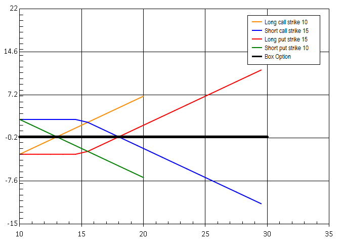
Combination of 4 basic legs, that achieves neutral interest rate position - riskless payoff.

• Long call strike 10
• Short call strike 15
• Long put strike 15
• Short put strike 10

The strategy has constant payoff, in ideal case the net premium paid for the strategy should be equal to the payoff. However the comission will reduce the profitability to nothing. Might be seen as a form of lending money on markets.

Barrier options

TODO!!!

Warrants

Warrants have the same parameters and behave just like options. There are few differences:

• They are not publicly traded, not listed, like OTC options.
• The expiration period is usually in years.
• Once the warrant is exercised the new outstanding shares of company are created. In case of options, no new shares are issued, the writer of the option has to buy them on the market.
• Often used as alternative to employees stock options.

Specifying option and it's price

This part is not about the actual pricing of options, that is determining the price. This is more about how options are exchanged on the market, in what units the prices as exchanged.

• Fixed price per contract
• In percentage
• Spread between legs
• Pricing by strike
• Total premium for multilegs

Forwards & Futures

By buying a forward or future, you have the right but also the obligation to buy given underlying at the selected price. Both are part of Delta One products. Since the price of the future moves the same way as the price of the underlying. Futeres unlikely to forwards are listed, standardized contracts. That means they can be bought on an exchange. Forwards are pure OTC products - not standardized at all.

Futures or Forwards have the same parameters as options, though in the majority of cases, no strike is specified. That is because the price at which the underlying will be exchanged at the expiration date, is defined solely by the market. Typically futures prices are listed on the market. For instance the current price of SPX Indice might be 2000 and the future which expires next month might be at 2050.

Pricing of futures

Futures are delta-one derivatives. The price of the future changes hand in hand with the price of the underlying (if the stock goes up one dolar, the future on the same stock in 3 months will go up as well by one dollar). That affects the way that futures are priced. Since typically the future price is always specicied with respect to the current stock price, there are 2 common ways of pricing futures:

TODO!!!

• Net Basis - the difference between stock price and future price is given by the broker in basis points.
• In Percentage - the future price is given as the percentage of current price. For bullish stock that will be greater than 100% and for bearish stocks that will be lower than 100%.

Future and Forward Rolls

Rolls enable the holder of given future to keep the position in the underlying when his future is about to expire.

Convertible Bonds, Reverse Convertible Bonds

These two derivatives at some point allow or force the holder to convert bonds into shares.

Convertible Bonds

Convertible Bond is a contract which allows the conversion of listed corporate bonds into the underlying equity. This is available only on listed companies that issue as well bonds to finance their operations. Converts are listed on exchanges. The companies issue the CBs just like the bonds the are underlying the converts.

From certain point of view, CB can be seen as an option, because if underlying stock behaves achieves certain performance, the owner will become the proprietary of the stock, if not, he will keep the bonds with regular return. For that reason, it makes sense to provide Delta while pricing Convertible Bonds, since the price of the CB will move with respect to the underlying share.

Convertible bond thus has the power of option and can be leveraged to obtain the underlying equity. It will be however more expensive than CALL option becase one pays for the bond as well.

Reverse Convertibles

Holder of a Reverse convertible is regulary paid a coupon as if he would be holding a standard bond. On the upside if the shares of the underlying company (and that can be any company, not just the issuer of the original bonds) fall bellow certain PUT like Strike. His bonds will convert into the stocks of this company

Swaps

Swaps as the name suggest are contracts that specify an exchange between the buyer and the seller of the contract. There are various types, depending on what is exchanged: Commodity, Interest Rate, Volatility or Variance.

Variance and Volatility Swaps

Volatility measures the magnitude of movements for given stock. Standard deviation is used to express the volatility of the stock. Variance is the square of standard deviation, so in a sense just amplified volatility.

Volatility or Variance swap allow the investor to bet on the volatility. The investor specifies a volatility level which he expects (striked volatility) and if the volatility goes over this level, he gets paid a bigger payoff. The payoff is specified as:

PayOff = VegaAmount (RealVolatility – Volatility Striked)/ RealVolatility

The bigger the difference between the Real Volatility and the Striked volatility is, more money does the buyer of such swap gets. The whole amount is multiplied by a multiplier called "Vega Amount". Vega is on of the greeks which meassures the sensitivity of an option to the change in the volatility of the option. There is however no connection here. It's just the term used on the markets for this multiplier.

Total Return Swaps

TRS allows the buyer to exchange the performance of certain stock for the performance of standard interest rate. The buyer can for instance bet on the performance of certain underlying (eg. MSFT stock) against a standard interest rate for standard period. For instance Euribor 6M is the interest rate provided by ECB (European Central Bank) for next 6M. That might be 2% fo example. The buyer believes that MSFT will beat that and asks the seller to pay him the difference if that is the case. The seller, for certain comission will do that. That allows the asset manager to bet on performance without owning the underlying shares.

ETFs

Exchange Traded Funds are compositions of stocks, that usually track an index or a sector. They are listed and traded like regular stocks. They companies that emit ETFs thus enable the asset managers to invest into whole sectors or regions, without the need of knowing the details of the markets.

Net Asset Value

Common to all funds which invest into stocks. At the end of the day the NAV of the fund is calculated as the sum of all the stocks own by the fund, divided by the number of shares.

ETFs however are listed themselves and traded on the market so beside the NAV they also have the market value. Their market value can be bellow or over the NAV.

Settlement date

The date when you need to the money to buy your ETF or when you will receive the money for selling. For ETFs it is 3 days after the deal (for some traditional reasons, I suppose).

Creation Redemption

Creation is the process of emission of ETF shares. ETF is supposed to track a sector or index and has exact composition. The company issuing ETFs needs to aquire the stocks that form the ETF to emit it. Since one share of ETF has exact composition, the issuer needs to aquire that exact amount to be able to sell that one share of ETF with certain comission.

Redemption is the reverse process. The issuer will buy the ETFs from the owners and give them back the underlying shares, or equal amount in cash.

This process is essential and allows the ETF to always trade around it's NAV. If the demand fo some ETFs (eg. ETF mirroring Asian construction market) would be too high, the prices would go up too much and get too far away from the real prices of the shares of the mirrored companies. The issuer can in that case emit more shares of the ETF. On the other hand if investors start to sell certain ETF too much and don't believe in the sector, the redemption process can reduce the quantity of the ETFs and stabilize the price which would go down too much otherwise.

Other crazy stuff

Autocallables

TODO!!!

Program Trading

An asset manager might interested in investing in sectors or countries, not exact shares. ETFs are one way to get there, Program Trading might be the other way. PT are basket trades (buying multiple underlyings in same time) and are very big in size, the buyer specifies the total amount of the traded volume (total notional) and might provide also the number of stock he wants to buy in the future. Then he gives multiple characteristics such as the percentage per country or sector. For instance 10% in US, 30% in UK and 25% in Telecom, 50% in services and so own. He also asks certain parameters such as how much this composition should track some index. This is done usually by setting the Beta in percent versus some index like SPX. The seller of such contract than provides price and some (huge) commission.

The investor will do such a trade when he wants to invest big amount of money in the same time to multiple markets. Usually the trade composition is determined by dedicated software, hence "Program Trading".

Neural Networks F#, XOR classifier and TSP Hopfield solver

It seems that recently thanks to the buzz around Deep Learning, Neural Networks are getting back the attention that they once had. This post contains just a very short introduction to Neural Networks, just enough to understand the F# code which follows. The aim for me is to learn F# and see how easy it can be to write Machine Learning code in F#.

I present here two examples of NN in F#:

• XOR classifier - sort of Hello World of NN. A simple composition of 2 input nodes, 2 hidden nodes and 1 output node which learns the XOR function.
• Solution to TSP using Hopfield NN. More complex network which evolves over time in it's configuration space to it's local minima, which shall correspond to optimal TSP tour.

Both working examples are available at my GitHub

Neural Networks

Artificial neural networks are computational models with particular properties such as the ability to adapt or learn, to generalise or to cluster and organise data. These models are inspired by the way that the human brain works. The building blocks of Neural Networks are inspired by Neurons - the building blocks of our brain. Neural Network can be seen as interconnected graph of nodes, where each node takes a role of a neuron. Each neuron can receive multiple signals, modify it and send it to other neurons to which it is connected. In this graph some vertexes are used to set the input, some of them are used to perform the computation and other onces will hold the output values.

Nodes are connected by edges which have different weights. The weight of the edge specifies how the signals is modified when passing from one node to another.

Perceptron

Perceptron is a basic block of linear neural networks. It is composed of multiple input nodes and a decision node. Perceptron is a single layer network. Input values are linked directly to the output node, connected by edges with certain weights.

The ouput node takes the incomming values, sums them and based on the result returns an output. The output could be binary or continous value. For instance a threashold can be used to say whether the output is 1 or 0.

In practice, very often the Sigmoid or also called logistic function is used to output value within the interval [0,1].

Linear separability

Single layer perceptrons can only learn linerearly separable data.

Imagine we want to separate a set of datapoints into multiple clusters. We visualize the data in 2-dimensional euclidian space. If we can separate the cluster by drawing direct line between the data points, the data is linearly seperable. The same can be applied on multi-dimensional data

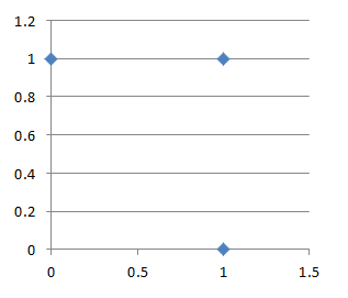
In a world of logical functions (we are building XOR classifier), this limitation means that a single layer perceptron is able to learn AND or OR function but it won't be able to learn XOR function.

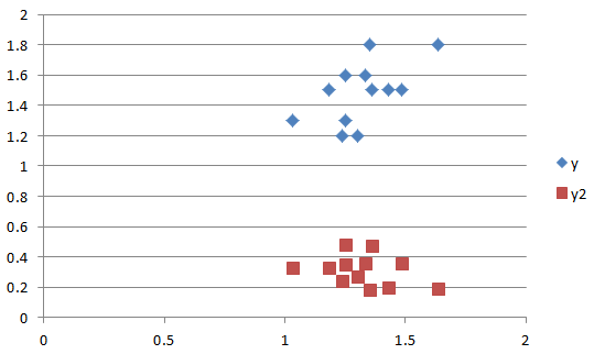
One can easily imagine a line that separates all OR positive results from the negatives once. On the other hand there is no streight line that separates the positive XOR results ([0,1] and [1,0]) from the negatives ([0,0] and [1,1])

Feed forward multilayer networks

Feed forward network can be thought as composition of perceptrons. Such network has one input layer, multiple hidden layers and one output layer. The feed forward network does not contain cycles, unlike the Hopfield network in the next examples (which is recurrent neural network).

Unlike single layer perceptron, multilayer feed forward network is capable of learning linerably non-separable data such as the results of XOR function.

XOR classifier

This is the first example. This network is called clasifier because it learns the XOR function. It can then "classify" the 2 values in the input into single value on the output.

Here is how the network looks like:

The NN diagram was drawn in latex, using the tkz-berge package. Look here if you want to know how.

The network starts with random weights and continously updates the weights so that the result in the output node corresponds to the XOR of input values. In order to update the weights Backpropagation (Backwards propagation of errors) technique is used.

The value of the output is compared to the real value (which is known). The error is determined as the differences between the output and the real value. Then the weights of the edges has to be updated to minimalize the error as shown later.

Implementation

Each layer can be represented as one dimensional array, the weights are stored using 2-dimensional array ([0,1] is the weight between nodes 0 and 1). Here is the function which calculates the sum of values incomming to a single node and passes the value to the activation function. The activation function here can be any function, as it is passed as parameter but here Sigmoid is used.

let pass (input:float[]) (weights:float[,]) activation =
let length = weights |> Array2D.length2
seq {
    for i in 0 .. length-1 do
        let sum = (Array.zip weights.[*,i] input) |> Array.sumBy (fun (v,w) -> v * w)
        yield activation sum
} |> Array.ofSeq

By applying the pass multiple times, the whole network can be composed as sequence of pass functions.

The training procedure

The following function is the main loop of the XOR network and we iterate over until we obtain good results and the network is adapted.

let train network rate input target =
    let n1 = completepass input network
    let delta = deltaOutput n1.output target
    let deltaHidden = passDelta n1.hidden delta n1.hiddenToOutput
    let updatedHiddenToOut = updateWeights n1.hidden delta n1.hiddenToOutput rate
    let updatedInToHidden = updateWeights n1.input deltaHidden n1.inputToHidden rate

Completepass just calls 2 times the pass function value and gets the input values trough the hidden layer to the output. The output is then compared to desired result and error is estimated. From this error an array of "delta" values per each output node is determined which is then used to update the weights.

In the case of XOR network, there is only one output, so the delta will one dimensional array.

The delta has to be propagated lower so that we can also update the weights between the input and hidden layer.

Backpropagating the error

First the error of each layer has to be calculated. In the example bellow the error of the output layer is the value (t-o) or (Target - Ouput). This value is multiplied by value o*(1-o) which is the derivation of the Sigmoid function. The resulting array contains for each node a delta value, which shall be used to adjust the weights.

let deltaOutput (output:array<float>) (target:array<float>) =
 (Array.zip output target) |> Array.map (fun (o,t) -> o * (1.0 - o) * (t - o))

Delta propagation

Calculating the delta value for the output layer is not sufficient to correct all the weights in the network, the delta has to be propagated to the lower layers of the network, so that we can update the weights on the input - hidden connections.

let passDelta (outputs:float[]) (delta:float[]) (weights:float[,]) =
    let length = weights |> Array2D.length1
    seq {
        for i in 0 .. length-1 do
            let error = (Array.zip weights.[i,*] delta) |> Array.sumBy (fun (v,w) -> v * w)
            yield outputs.[i] * (1.0 - outputs.[i]) * error
    } |> Array.ofSeq

The "error" of the hidden layer is just the delta multiplied by the weight associated to the edge that propagates this delta to the lower value.

The last missing piece is the function that woudl update weights between 2 layers.

let updateWeights (layer:float[]) (delta:float[]) (weights:float[,]) learningRate =
    weights |> Array2D.mapi (fun i j w -> w + learningRate * delta.[j] * layer.[i])

Learning rate is a constant that determines how quickly the edges are updated. If the learning rate is too big, the network might miss the optimal weights. However if it is too small it will take longer time to get to the correct solution.

At the beginning the weight are set to random values between 0 and 1, or slided slightly. From the quick tests that I did it seems that for instance using learning rate of 0.3 it took 20000 iterations to get to a neural network that would XOR the values on it's inputs.

Hopfield-Tank network and Travelling Salesman Problem

TSP is one of the well known Combinatorial optimization problems and as such, it has been solved in many different ways (Integer Linear Programming, Genetic or Biologically inspired algorithms and other heuristics). Neural Networks are one of the many approaches to provide a solution to this problem.

Even within Neural Networks several different approaches have been developed to solve TSP (eg. elastic nets,self-organizing map). The approach demonstrated here is the oldest one: Hopfield neural network.

Hopfield neural network

Hopfield NN is a recurrent neural network (connections in the network form cycles). The units (nodes) in a Hopfield network can have only 2 values: 0|1 or -1|1 depending on literature, but in either case values that encode a binary state. The network is fully connected (each node is connected with any other node). The connection matrix is symetric, that is the weights on the edges are the same in both directions.

The initial Hopfied network had only binary values (0/1) but to solve TSP and for other problems continous version of the network is used, where every node has value in range [0,1].

The value of each node depends on the input potential of the node (Ui) and in order to keep it between (0,1) the tanh function is used:

The value of the input potential of each node depends on the values of all nodes that are connected to it and the values of the connections weights. This is actually identical to the way that the nodes in the XOR classifier behaved.

Network energy

Each state of the HNN can be described by a single value called Energy. While iterating and changing the state, the energy of HNN will either stay the same or will get smaller. The energy of the network will evenutelly convert to a local minimum - the state of the HNN that we target to solve the TSP

Hopfiled approach to TSP

The first and original approach to solve TSP was described in 1985 by Tank and Hopfield in their paper "Neural Computation of Decisions in Optimization Problems". Since then many more attempts were made. I have found these few papers or surweys available online quite useful and have used them to deduce my implementation:

• Jean-Yves Potvin - The Traveling Salesman Problem: A Neural Network Perspective
• Perspective of a neural optical solution of the Traveling Salesman optimization Problem
• Jacek Mandziuk -Solving the Travelling Salesman Problem with a Hopfield - type neural network

If I should pick one, I would say that the first one gave me most information about the problem, event though not enough implementation details. The others once then made it (almost) clear how to implement the solution.

Encoding TSP in Hopfield network

The neural network used to encode the TSP and it's solution is square matrix of nodes having N rows (one for each city) and N columns (one for each position in the tour), where N is the number of cities. When the algorithm finishes and the network converges to it's final state, each node will have value of either 0 or 1. As said the network in fully inter-connected so there is an edges between each node, which is not shown in the image bellow.

If the node in i-th row and j-th column has value 1, the city (i) will be in the tour on position (j).

As described above the network evolves and each node changes it's value over time. The secret of the algorithm is thus to provide such update rule that at the end the matrix of nodes will follow these criteria:

• Only one node in each row will have value 1
• Only one node in each column will have value 1
• There will be exactly N nodes having value 1
• The distances of the tour will be minimal

To come up with such update rule, Energy function has to be determine which will attain it's minimum for optimal solution of TSP. The energy function has to take into account the above specified rules. The following definition will satisfy the rules. Note that the following equations were taken from the J.Y Potvin's - paper

A,B,C and D are constants and the 4 sumations here correspond to the 4 above mentioned points.

Describing the dynamic of the network

There are two ways to describe the behaviour and the dynamic of the network:

• From the TSP energy function and the standard Hopfield network energy function we determine the weights between the nodes. Then we can let the network evolve over time. Since we have the weights of the connections between the nodes, we could iterate over the nodes, sum all the weighted inputs and set the output of the node. That would be an approach similar to the one taken on the XOR. This has one disadvantage, that is that the connection weights have to be determined from the equality between the standard Hopfield model enery function and the TSP Hopfield model function. There is an easier way without determining the connections weights.
• The easier way is to describe the change of the input potential without determining the weights of the edges. Then we can just iterate or randomly choose nodes, determine the new value of the potential and update the values of the connected nodes. This seems maybe ackward, because the network will evolve without having specific weighed connections between nodes. This options is described further.

The change in the node's input potential

One of the definition of the input potential of a node (i) can be described by:

What we want to determine, is how this value will change over time, when the network evolves. The change of the potential over time is it's partial derivation with respect to the time.

When doing a computer simulation we will described the value of Ui in time T+1, or here T+ delta t. Where delta T is some small time interval.

This equation is at the hearth of this algorithm. We now have an exact specification of what the value of potential Ui will be in time T+1. That is our iterating algorithm has to perfrom exactly this updated.

Implementation details

• Compute the distance matrix, containing the distance between each 2 cities
• Initialize the network with random values
• Pick randomly a node, compute the change in the input potential
• Update the value of the node from the input potential change
• Every n-iterations calculate the energy of the network
• Once the energy of the network stabilizes or you have reached fixed number of iterations - stop the process
• Translate the network into a city path

The network can be stored in 2-dimensional matrix. One can choose between storing the input potential of each node or the value of the each node, because the value of the node can be calculated from the potential at any time. I have chosen the second option and I store the input potential two dimensional array u.

The following code is the calculation of the input potential change of single node at coordinates (city,position). This is just retranscription of the equation above.

let singlePass (distances:float[,]) (u:float[,]) pms city position = 
    let n = Array2D.length2 u
    
    let values = u |> toValues pms

    let aSum = sumAllBut position (values |> rowi city)

    let bSum = sumAllBut city (values |> coli position)
            
    let cSum = (values |> Seq.cast<float> |> Seq.sum) - float(n+1)

    let dSum = dSumCalc distances city position values

    let dudt = -pms.A*aSum - pms.B*bSum - pms.C*cSum - pms.D*dSum
    //value of input potential in t+ delta_t
    let r = u.[city,position] + pms.dTime*(-u.[city,position] + dudt)
 //Alternatively according to the paper by Jacek Mandziuk one can just use the update value
 //let r = dudt
    r

There are few things to note. This code takes the distances matrix, the current state of the network (the value of input potential of each node), parameters of the network (constants A,B,C,D from equations above) and row (city) and the column (position) of the node that we are updating. The toValues method takes the current value of each node potential and returns a matrix of node values. The rowi and coli method return respecively one row or one column from 2 dimensional array. The sumAllBut method adds all elements of one-dimensional array except an element at position which is passed to the method. The dSumCalc method is the only one with a bit more compexity and it calculates the D value of the equation above (the one that assures the minimalization of the TSP circuit)

let rowi row (network:float[,]) = 
    network.[row,*] |> Array.mapi (fun j e -> (e,j))

let coli col (network:float[,]) = 
    network.[*,col] |> Array.mapi (fun j e -> (e,j))

let sumAllBut (i:int) (values:(float*int)[]) = 
    Array.fold (fun acc (e,j) -> if i<>j then acc + e else acc) 0.0 values

let dSumCalc distances city position (v:float[,]) = 
    let n = v |> Array2D.length1
    (distances |> rowi city) |> Array.sumBy (fun (e,i) -> 
        let index1 = (n+position+1) % n
        let index2  = (n+position-1) % n
        e*(v.[i,index1] + v.[i,index2])
    )

let toValues (pms:HopfieldTspParams) u = 
    u|> Array2D.map (fun (ui) -> v ui pms)

//calculates the value of node from input potential
let v (ui:float) (parameters:HopfieldTspParams) = (1.0 + tanh(ui*parameters.alfa))/2.0

The method which updates the input potential of single node can be called in 2 different ways. Either we pick the nodes randomly multiple times or we loop over all the nodes serially. If the update is serial then the only random element of the algorithm is the initialization of the netwok.

let serialIteration u pms distances = 
    u |> Array2D.mapi (fun i j x -> singlePass distances u pms i j)

let randomIteration u pms distances = 
    let r = new Random(DateTime.Now.Millisecond)
    let n = Array2D.length1 u
    for i in 0 .. 1000*n do
        let city = r.Next(n)
        let position = r.Next(n)
        u.[city, position] <- singlePass distances u pms city position
    u

The random iteration here is repeated 1000*n times where n is the number of cities, which is probably more than enough since the network seems to converge much sooner. Just for the sake of completeness, here is the method that runs 10 times either serial or random iteration.

let initAndRunUntilStable cities pms distances = 
    let u = initialize cities pms
    {1 .. 10} |> Seq.fold (fun uNext i -> 
            match pms.Update with
                | Random -> randomIteration uNext pms distances
                | Serial -> serialIteration uNext pms distances
    ) u

And here high level method, that generates a random example of TSP problem, calculates distances between all cities and runs the algorithm until a stable and correct solution is found. That is until the network returns feasable solution.

let sampleRun (pms:HopfieldTspParams ) (n:int) =
    let cities = generateRandomCities n
    let distances = calculateDistances cities
    let networks = Seq.initInfinite (fun i -> initAndRunUntilStable cities pms distances)
    let paths = networks |> Seq.map (fun v-> currentPath v)
    let validPath = paths |> Seq.find (fun path -> isFeasable path)
    cities, validPath

Results

The results are not overwhelming, on the other hand I have only implemented the most simple version of the algorithm. In the original paper the authors stated that the convergence rate to feasable solutions was about 50%. But depending on the parameters one can get better results. See bellow one of the runs of the algorithm on 6 random nodes.

Here is the complete list of parameters for Hopfield network and the values that I ended up using:

• Alpha: the parameters which shapes the Sigmoid decision function applied on each node (500)
• A: input potential change function, sum of rows (500)
• B: input potential change function, sum of columns (500)
• C: input potential change function, max N cities (200)
• D: input potential change function, minimalization of tour length (300)
• dTime: represents the delta T, the small update in time for each update of the input potential value (0.00001)

I have also used the standard update rule to obtain new value of the input potential which takes into account the current input potential.

     let dudt = -pms.A*aSum - pms.B*bSum - pms.C*cSum - pms.D*dSum
    //value of input potential in t+ delta_t
    u.[city,position] = u.[city,position] + pms.dTime*(-u.[city,position] + dudt)

According to the paper by Jacek Mandziuk one can just use the updated values as the new input potential, so that the update rule would become only:

    let dudt = -pms.A*aSum - pms.B*bSum - pms.C*cSum - pms.D*dSum
    u.[city,position] = dudt;

This rule didn't work for me. The convergance rate wasn't better neither were the tours lengths. Of course for such version, different values for network parameters have to be used.

Note that GitHub repostity and specifialy the Hopfield module contais more code:

• Method to determine the correct parameters. The performance of the algorithm greatly depends on the parameters of the Energy function and on the parameter alfa, which amplyfies the effect of the input potential on the value of given node.
• Few lines are also available to draw the solution using Windows Forms Charts, through F#

FSharp.Data and Unit Testing issues

I have recently run into two separate issues while testing some F# data providers based code. I am using ReSharper's NUnit runner and sometimes NCrunch.

NCrunch issues

NCrunch won't compile your solution when FSharp.Data is referenced. This component internally references FSharp.Data.DesignTime which has to be avaiable for the compilation - and NCrunch does not have those libs available, because the DLL is not referenced the standard way, but must be provided by Visual Studio.

The current solution is to reference FSharp.Data.DesignTime manually. If you are using nuget, than the DLL can be found in the pacakages foder as shown bellow:

Note that I have tested and had the same issue with FSharp.Data 2.1.0 and 2.2.0.

NUnit runner issues

NUnit did load the test correctly, but the test failed with SystemMissingMethodException

Luckily the solution can be found on StackOverflow and was caused by the tested library being Portable Class Library instead of standard F# library.

Events visualization with EvenDrops and KoExtensions (D3 and Knockout)

I have recently needed to visualize a set of events which occurred within a certain interval. Each event would have couple parameters and there would be multiple event lines. Let's say that you want to visualize the occurences of car sales in couple countries. For each sale you would also want to visualize the price and the mark of the sold car. Before writing everything from scratch, I have found EventDrops project which responded to the majority of my requirements. It had just one flaw and that is that there is no way to chart another characteristics for each event.

I have decided to add such possibility and since I am using KnockoutJS and binding to create all of my charts I have also decided to add EventDrops to my KoExtensions project - in order to make it's usage simplier. The resulting chart looks like this:

This example is available on GitHub as part of KoExtensions.

What I have added to the original event drops are the following possibilities:

• The chart now accepts generic collection instead of just a collection of dates. The developer in turn has to specify a function to get the date for each item
• The size of the event is dynamic
• The color of the event is dynamic
• Better possibility to provide a however action
• The size of the event can use logarithmic or linear scale
• Everything is available as KnockoutJS binding

The html is now really straightforward:

<div data-bind="eventDrops: carSales, chartOptions: carSalesOptions"></div>

The javascript behind this page contains a bit more to generate the data:

require(['knockout-3.2.0.debug', 'KoExtensions/koextbindings', 'KoExtensions/Charts/linechart', 'KoExtensions/Charts/piechart', 'KoExtensions/Charts/barchart'], function(ko) {
 function createRundomSales(country) {
  var event = {};
  var marks = ['Audi', 'BMW', 'Peugot', 'Skoda'];

  event.name = country;
  event.dates = [];
  
  var endTime = Date.now();
  var oneMonth = 30 * 24 * 60 * 60 * 1000;
  var startTime = endTime - oneMonth;

  var max = Math.floor(Math.random() * 80);
  for (var j = 0; j < max; j++) {
   var time = Math.floor((Math.random() * oneMonth)) + startTime;
   event.dates.push({
    timestamp: new Date(time),
    carMark: marks[Math.floor(Math.random() * 100) % 4],
    price: Math.random() * 100000
   });
  }

  return event;
 }


 function createSales() {
  var sales = [];
  var countries = ['France', 'Germany', 'Czech Republic', 'Spain'];
  countries.forEach(function(country) {
   var countrySales = createRundomSales(country);
   sales.push(countrySales);
  });
  return sales;
 }

 function TestViewModels() {
  var self = this;

  self.carSales = ko.observableArray([]);
  self.carSales(createSales());

  self.carSalesOptions = {
   eventColor: function (d) { return d.carMark; },
   eventSize: function (d) { return d.price; },
   eventDate: function (d) { return d.timestamp; },
   start: new Date(2014, 8, 1)
  };
 }

 var vm = new TestViewModels();

 ko.applyBindings(vm);
});

In this example the createSales and createRandomSales methods are just use to get testing data. Once the testing data is generated it is stored to the carSales observable collection. Any time this collection is changed the chart would be updated.

The sales collection looks a bit like this:

The carSalesOptions object contains the charting options. These tell to the event drops chart the necessary information to specify how big and which color should be used for the given event.

Unit testing Knockout applications

In ideal case any View Model in Knockout based application should be completely unit-testable. The View Model ofcourse interacts with other code but in majority of cases this would be either some UI code or the server side code, probably over REST API. The UI interaction should be minimal. If possible, the binding capabilities of Knockout should be leveraged. The REST API is not available while unit testing and thus has to be mocked or hidden by an abstraction layer. I went for the first option and this blog describes how to mock the AJAX calls while unit testing Knockout View Models. At the end I also provide information about the ChutzPah test runner and the way that the tests can be run from within Visual Studio.

The typical view model that I am using looks like the following one.

function AssetViewModel(){
    var self = this;
    self.city = ko.observable();
    self.country = ko.observable();
    self.size = ko.observable();
  
    self.load = function(){
        $.ajax("/api/assets/" + self.city(), {
            data: dto,
            type: "GET", contentType: "application/json",
            success: function (result) {
                self.updateData(data);
            }
        });
    }

    self.save = function () {
        var dto = self.toDto();
        self.isBusy(true);
        self.message("Saving...");

        $.ajax("/api/assets/", {
            data: dto,
            type: "POST", contentType: "application/json",
            success: function (result) {
                self.edit(false);
                self.isBusy(false);
                self.message(result.message);
                self.update(result.data);
            }
        });
    };

    self.update = function(updateData){
        self.city(updateData.City);
        self.country(updateData.Country);
    }
 
    self.toDto = function () {
        var model = new Object();
        model.City = self.city();
        model.Country = self.country();
        return JSON.stringify(model);
    };
}

You might thing that the toDto method is useless if one uses the Knockout Mapping plug-in, however in many cases the view models get much more complex and they can't be directly mapped to any kind of data transfer objects or domain objects. Other than that, nothing should be surprising here. The save method sends the dto over the wire and than treats the response.

The unit test

Nowadays one has a choice between multiple JavaScript testing frameworks, QUnit, Jasmine or Mocha being probably the most common choices - I am staying with QUnit. Testing the updateData with QUnit might look like this.

var vm;
function initTest() {
    
    var vm = new AssetViewModel();
}

$(function () {

    QUnit.module("ViewModels/AssetViewModel", {
        setup: initTest
    });

    QUnit.test("updateData sets correctly the city", function () {
        var data = {
            City: "Prague",
            Country:"Czech Republic"
        };
        vm.updateData(data);
        equal(vm.city(), "Prague");
    });
}

QUnit module function takes 2 parameters - name and a sort of configuration object. Configuration object can contain a setup and tearDown methods. Their usage and intend should be clear.

This test case is very simple for 2 reasons: it does not depend on any external resources and it executes synchronously.

QUnit has 3 assert methods which can be used in the tests:

• ok - One single argument which has to evaluate to true
• equal - Compare two values
• deepEqual - Recursively compare a objects properties

Asynchronous testing

Here is the test for the save method which calls the REST server interface.

function initTest() {
      $.mockjax({
        url: '/api/assets/Prague',
        type: 'GET',
        responseTime: 30,
        responseText: JSON.stringify({
            Name: "Prague",
            Country: "Czech Republic",
            Size: 20
        })
    });
}

$(function () {

    QUnit.module("ViewModels/AssetViewModel", {
        setup: initTest
    });

    QUnit.asyncTest("testing the load method", function () {    
        setTimeout(function () {
            ok(true, "Passed and ready to resume!");
            start();
            vm.load();
            QUnit.equal(vm.size(),20);
        }, 100);
    });
}

I am using MockJax library to mock the results of the REST calls. The initTest method setups the desired behavior of the REST service call, the test is executed after 100ms of waiting time. In this case the call is a GET and we define the response simply as JSON data. QUnit has a method for asynchronous tests called asyncTest.

Currently there is a small issue in MockJax regarding the way that incoming JSON values are handled. That might get fixed in future versions.

Mocking the server interface

Returning a simple JSON data may be sufficient for some case, for others however we would maybe like to verify the integrity of the data sent to the server, just like when testing the save method

var storedAssets = [];
function initTest() {
      $.mockjax({
        url: '/api/assets',
        type: 'POST',
        responseTime: 30,
        response: function (data) {
            storedAssets.push(JSON.parse(data.data));
        }
    });
}

$(function () {

    QUnit.module("ViewModels/AssetViewModel", {
        setup: initTest
    });

    QUnit.asyncTest("save asset - check the update of the size", function () {
        vm.size(10);
        vm.save();
        setTimeout(function () {
            ok(true, "Passed and ready to resume!");
            start();
            equal(storedAssets.length, 1);
            var storedAssets = storedCharges[0];
            equal(storedAssets.Size, vm.size());
        }, 100);
    });
}

In this case the save method passes the JSON data to the server side. The server is mocked by MockJax which only adds the data to a dump array, which can be then used to verify the integrity of the data.

Running Unit Tests in Visual Studio

There are 3 reasons for which I am using Visual Studion even for JavaScript project:

• Usually the application has some backend written in .NET and I don't want to use 2 IDEs for one single application.
• I can easily debug JS application from within VS. Of course Chrome's debugger is very useful as well - but if I can do everything from 1 IDE, why should I use other.
• ReSharper has really good static analysis of JavaScript and HTML files. That saves me a lot of time - typos, unknown references and other issue are catched before I run the application.
• I can run JavaScript unit tests right from the IDE.

To run the Unit Tests I am using ChutzPah test runner. ChutzPah internally uses the PhantomJS in-memory browser, and interprets the tests. While using this framework, one does not need the QUnit wrapper HTML page and the Unit Tests can be run as they are.

Note that ChutzPah already contains QUnit and you will obtain TimeOutException, if you try to add a reference to QUnit explicitly (http://chutzpah.codeplex.com/workitem/72).

Since your tests are just JavaScript files, without the HTML wrapper page, ChutzPah needs to know what libraries do your View Models reference and load them. This is handled using a configuration file chutzpah.json which has to be placed alongside the unit tests. The following is an example of configuration file that I am using for my tests.

{
    "Framework": "qunit",
    "References" : [
        { "Path": "../Scripts/jquery-2.1.0.js"},
        { "Path": "../Scripts/knockout-3.1.0.js"},
        { "Path": "../Scripts/jquery.mockjax.js"},       
        { "Path": "../Scripts/tech", "Include": "*.js"},
        { "Path": "../ViewModels", "Include": "*.js"}
    ]
}

JSON DateTime serialization

This is more a side note. Dates in JSON are serialized into ISO format. That is good, the problems is that if you try to deserialize an object which contains a date, the date comes out as a string. The reason of course is that since there is no type, the de-serializer does not know that given property is a date - and keeps the value as a string. You can read more on dates serialization in JSON here. Any time that you are mocking backend which handles dates you have to be aware of this fact. Remember the mock of the back-end which inserts the object to a dummy array that I have used above:

function initTest() {
      $.mockjax({
        url: '/api/assets',
        type: 'POST',
        responseTime: 30,
        response: function (data) {
            storedAssets.push(JSON.parse(data.data));
        }
    });
}

JSON.parse call we handle the dates as strings. If the ViewModel has a date property, you will have to convert it into string before testing the equality.

Detecting extreme values in SQL

In a set of data points, outliers are such values that theoretically should not appear in the dataset. Typically these can be measurement errors or values caused by human mistakes. In some cases outliers are not caused by errors. These values affect the way that the data is treated and any statistics or report based on data containing outliers are erroneaus.

Detecting these values might be very hard or even impossible and a whole field of statistics called Robust Statistics covers this subject. If you are further interested into the subject please read Quantitative Data Cleaning For Large Databases written by Joseph M. Hellerstein from UC Barkeley. Everything that I have implemented here is taken from this paper. The only thing that I have added to that are two aggregates for SQL Server which help efficiently get the outliers and extreme values from the data stored in SQL Server and a simple tool to chart data and distribution of data using JavaScript

Theory

Any dataset can be characterized by the way the data is distributed over the whole range. The probability that a single point has given value in the dataset is defined using the probability distribution function. The Gaussian standard distribution is only one among many distribution functions, I won't go into statistics basics here, but let's consider only the standard distribution for our case.

In the Gaussian distribution the data points are somehow gathered around the "center", and most values fall not far. Rare are the values really far away from the center. Intuitively the ouliers are points very far from the center. Consider the following set of numbers which represent in minutes the length of a popular song:

3.9,3.8,3.9,2.7,2.8,1.9,2.7,3.5, 4.4, 2.8, 3.4, 8.6, 4.5, 3.5, 3.6, 3.8, 4.3, 4.5, 3.5,30,33,31

You have probably spotted the values 30,33 and 31 and you immediately identify them as outliers. Even if the Doors would double the length of their keyboard solo we would not get this far.

The standard distribution can be described using the probability density function. This function defines the probability that the point will have given value. The function is defined with two parameters: the center and the dispersion. The center is the most common value, the one around which all others are gathered. The dispersion describes how far the values are scattered from the center.

The probability that a point has a given value, provided that the data has the Gaussian distribution is given by this equation:

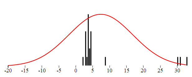
We can visualize both the theoretical and the real distribution of data. The distribution probability density function is continuous and thus can be charted as simple line. The distribution of the real data in turn can be visualized like a histogram.

The following graphics were created using KoExtensions project, which is a small mediator project making Knockout and D3 work nicely together.

In perfect world the center is the mean value. That value is probably not a part of a data set but represents the typical value. The seconds measure which describes how far from the center the data is dispersed is called standard deviation. If we want to obtain the standard deviation from data we take the distance of each point from the center, square these values add them together and take square root. So we actually have all we need to get the distribution parameters from the data.

This approach of course has one main flaw. The mean value is affected by the outliers. And since the dispersion is deduced using the mean and outliers affect the mean value, the dispersion as well will be affected by them. In order to get a description of the dataset not affected by the extreme values one needs to find robust replacements for the mean and the dispersion.

Robust Center

The simplest and very efficient replacement for the mean as the center of the data is the median. Median is such value that half of the points in the dataset are smaller are bellow. That is if the data set consists of even number of samples, we just need to order the values and take mean of the two values in the middle of the ordered array. If the data consist of odd number of values then we take the element exactly in the middle of the ordered data. The before mentioned paper describes two more alternatives: trimmed mean, winsorized mean. Both of these are based on the exclusion of marginal values and I did not used them in my implementation.

Let's take the median of the given dataset and see if the distribution function based on it fits better the data. Even though the center is now in correct place the shape of the function does not fit completely the data from the histogram. That is because the variance is still affected by the outliers.

Robust Dispertion

Standard variance takes into account the the distance of all the numbers from the center. To rule out the extreme values, we can just use the median of distances. The outlier's distance from the center is much bigger than other distance and by taking the median of all distances we can get rid of outlier's influence over the dispersion. Here is the distribution function using this Robust type of dispersion. This characteristic is called MAD - Median Absolute Deviation.

Detecting the outliers

Now that we have the value of "real" center and "real spread" or dispersion we can state that the outlier is a value which differs "too much" from the center, taking into account the dispersion. Typically we could say that the outliers are such values that have a distance from center greater or equal to 10 * dispersion. The question is how to specify the multiplication coefficient. There is a statistics method called Hampel Indetifier which gives a formula to obtain the coefficient. Hampel identifier labels as outliers any points that are more than 5.2 away from the MAD. More details can be found here.

The overall reliability of this method

A question which might arise is up to which kind of messy data this method can be used. A common intuition would say that definitely more than the half of the data has to be "correct", in order to be able to detect the incorrect ones. To be able to measure the robustness of each method of detecting outliers, statisticians have introduced a term called Breakdown point. This point states which percentage of the data can be corrupted in order for given method to work. Using the Median as the center with the MAD (Median Absolute Deviation) has a breakdown point of 1/2. That is this method works if more than half of the data is correct. The standard arithmetic mean has a BP = 0. It is directly affected by all the numbers and one single outlier can completely move the data.

SQL implementation

In order to implement detection of outliers in SQL, one needs to first have the necessary functions to compute the mean, median and dispersion. All these functions are aggregates. Mean (avg) and Dispersion (var) are already implemented in SQL Server. If you are lucky enough to use SQL Server 2012 you can use the built-in median aggregate as well. The robust dispersion however has to be implemented manually even on SQL Server 2012.

Implementing aggregates for SQL Server is very easy, thanks to the predefined Visual Studio template. This templates will create a class for you which implements the IBinarySerializable interface and is decorate with couple attributes defined in the Microsoft.SqlServer namespace.

This class has 4 important methods:

• Init - anything needed before starting the aggregation
• Accumulate - adding one single value to the aggregate
• Merge - merging two aggregates
• Terminate - work to be done before returning the result of the aggregate

Here is the example of the Median aggregate

private List ld;

public void Init()
{
    ld = new List();
}

public void Accumulate(SqlDouble value)
{
    if (!value.IsNull)
    {
        ld.Add(value.Value);
    }
}

public void Merge(Median group)
{
    ld.AddRange(group.ld.ToArray());
}

public SqlDouble Terminate()
{
    return Tools.Median(ld);
}

Note that some aggregates can be computed iteratively. In that case all the necessary logic is in the Accumulate method and the Terminate method can be empty. With Median this is not the case (even though some iterative estimation methods exist. For the sake of the completeness, here is the implementation of median that I am using. It is the standard way: sorting the array and taking the middle element or average of the two middle elements. I am returning directly SqlDouble value, which is the result of the aggregate.

public static SqlDouble Median(List ld)
{
    if (ld.Count == 0)
        return SqlDouble.Null;

    ld.Sort();
    int index = ld.Count / 2;

    if (ld.Count % 2 == 0)
    {
        return (ld[index] + ld[index - 1]) / 2;
    }
    return ld[index];
}

Implementing the Robust variance using the MAD method is very similar, everything happens inside the Terminate method.

public SqlDouble Terminate()
{
    var distances = new List();
    var median = Tools.Median(ld);

    foreach (var item in ld)
    {
        var distance = Math.Abs(item - median.Value);
        distances.Add(distance);
    }

    var distMedian = Tools.Median(distances);
    return distMedian;
}

That implementation is directly the one described above: we take the distance of each element from the center (median) and than we take the median of the distances.

Outliers detection with the SQL aggregates

Having implemented both aggregates, detecting the outlier is just a matter of a SQL query - giving all the elements which are further away from the center than the variance multiplied by a coefficient.

select * from tbUsers where Height > ( Median(Height) + c*RobustVar(Height)) or Height < (Median(Height) - c*RobustVar(Height))

You will have to play with the coefficient value c to determine which multiplication gives you the best results.

JavaScript implementation

The same can be implemented in JavaScript. If you are interested in a JavaScript implementation you can check out the histogram chart from KoExtensions. This charting tool draws the histogram and the data distribution function. You can than configure it to use either Median or Mean as the center of the data as well as to use MAD, or standard variance to describe the dispersion.

KoExtensions is based on Knockout.JS and adds several useful bindings and the majority of them to simplify charting. Behind the scenes the data is charted using D3.

To draw a histogram chart with the distribution and detecting the outliers at the same time one needs just few lines of code

<div id="histogram" data-bind="histogram: data, chartOptions : {
        tolerance : 10,
        showProbabilityDistribution: true,min : -20,
        expected: 'median',
        useMAD: true,
        showOutliers: true}">

var exData = [3.9,3.8,3.9,2.7,2.8,1.9,2.7,3.5, 4.4, 2.8, 3.4, 8.6, 4.5, 3.5, 3.6, 3.8, 4.3, 4.5, 3.5,30,33,31];
  
function TestViewModel() {
    var self = this;
    self.data = ko.observableArray(exData);
}

var vm = new TestViewModel();
ko.applyBindings(vm);
initializeCharts();

Knockout.JS is a JavaScript MVVM framework tool which gives you all you need to create bi-directional binding between the view and the view model, where you can encapsulate and unit test all your logic. KoExtensions adds a binding call "histogram", which takes simple array and draws a histogram. In order to show the probability function and the outliers one has to set the options of the chart as shown in the example above.

Introduction to GPU programing through AMP C++

Few months ago I tried to learn a bit about GPU programming and I took notes a started to write this post. I am publishing this now even though it's not complete, however being too busy, I am not sure whether I will have the time to get back to this later.

Since couple years CUDA (*2007) and OpenCL (*2008) have established themselves as standard frameworks for parallel programming on the GPU. In 2011 new framework came to the landscape of GPGPU programming, which does not compete on the same level, but rather represents new abstraction between the GPU and the developer.

AMP stands for Accelerated Massive Parallelism and it is an open C++ standard. The implementation of AMP provided by Microsoft consists of three main features:

• C++ language features and compiler
• Runtime
• Programming framework containing classes and functions to facilitate parallel programming

As well as OpenCL and unlike CUDA, AMP is a standard not only for GPU programming but for any data-parallel hardware. Typical example of such a hardware is the vector unit of standard CPU, capable of executing SIMD (Single Instruction Multiple Data) instructions. Or in the near future a cloud based cluster. AMP is an abstraction layer which can be used to target different devices from different vendors.

The following diagram depicts how AMP C++ fits to the world of GPGPU programming.

Microsoft has implemented AMP on top of DirectCompute technology and it is the only production ready implementation. Currently there are also two Proof Of Concepts AMP implementations Shelvin park project done by Intel and open source modification of the LLVM compiler (more information here). Needless to say that the adoption of such standard will depend a lot on whether these implementations will be taken further and whether we will have real implementation based on CUDA.

First look at the code

Without further introduction let's take a look at the classical "Hello World" of GPGPU programming: Addition of elements of two vectors (here without the boiler plate code).

parallel_for_each(e,[=](index<2>idx) restrict(amp){
 c[idx] = a[idx] + b[idx];
});

If you have ever tried out OpenCL or CUDA, you should find this piece of code less verbose and quite easy to read. That is the result of the main ideas behind AMP C++:

• Full C++ - unlike CUDA or OpenCL, AMP is not a C like dialect.
• Minimalist API - AMP hides as much as it can from the developer.
• Future proofed - the API is designed for heterogeneous programming. In the future GPU should be only one of it's usages. It aims to be a standard for programming on distributed systems.

Before going futher with more examples we have to provide basic description of GPU architecture as it is crutial to understanding certain parts of AMP

GPU architecture

Here I will give a high level overview of the GPU architecture. If you are already familiar with the GPU architecture, feel free to skip this section.

Currently there are two main producers of GPU chips: NVidia and ATI (AMD). A little behind comes Intel. Each of them constructs graphic cards with different architecture. Moreover the architectures change significantly with the realease of any new version. Nevertheless certain concepts are shared by all of them. I will describe here shortly the NVidias Fermi and ATIs Cypress architecture. The succesor of Fermi is called Kepler.

Processor architecture

The GPU is composed of hundreds of pipelined cores. The cores are grouped to computation units. NVidia calls these units Symmetric Multiprocessors. Each computation unit is assigned a unit of work.

ATI uses slightly different abstraction. Similary to NVidia the "cores" are grouped to Symmetric Multiprocessors, however each core is called Thread Processor and is a capable of executing VLIV (Very Long Instruction Word) instructions. It has therefore 4 arithmetic logical units and one Special Function Unit. The compiler has to find independent operations and construct the VLIW instruction. If the compiler is not able to find these independent operations than one or more of the ALUs will not be performing any operation.

Memory access

The GPU has a global memory which can be accessed by all cores. This access is quite costly (hundreds of cycles). Each simetric multiprocessor in turn has a small scratch-pad memory which is called usually local memory. This memory can be accessed only by the threads running on the given SM. The access to local memory is much cheaper (around 10 cycles). This memory can either take a role of a cache or can be managed by the developer directly. In addition each core has its own general purpose registers, used to perform the computations.

GPUs usually run computations on data which is accessed only once, unlike CPUs where the same memory pages are often used repetively. For this reason it is better for the developer to control the local memory. That's why historically the local memory did not act as cache on GPUs. However this will probably change in the future, and some form of caching will be provided by the GPU directly.

Scheduling

Scheduling is essential because it allows the effective usage of the processor. Since the memory access is expensive, other operations might be executed while the processor is waiting for the data to come. NVidia processors have "costless" context switching, so while one thread is blocked other can take over. Therefore the number of threads scheduled might affect the computation performance, while if not enough threads are available for scheduling some might be waiting for the memory page loads.

The programming models comparison:

These architectural concepts are used by NVIDIA and ATI. Each of the 3 GPU programming models (CUDA, OpenCL, AMP) can has its own dialects and namings. The following table shows the terms used by all three technologies. We will discuss the AMP terms used in this table later in the article.

Term	CUDA	AMP C++	OpenCL
Basic unit of work	thread	thread	work-item
The code executed on one item	kernel	kernel	kernel
The unit processing one group of working units	Streaming multiprocessor	-	Compute unit
Cache-style memory accessible by grouped threads	shared memory	tile static memory	local memory
Group of working units sharing local memory	warp	tile	work-group

The tools offered by each framework

Now when the architecture of GPU has been described we can define the tools which each framework needs to provide. In the next part of the article I will try to describe how AMP adresses these issues.

• Tell the compiler which part of the code will be offloaded to the GPU
• Provide constructs to work with multidimensional vectors
• Provide a way to transfer the data between the GPU and the CPU
• Give the developer tools to write efficient programs. That is to address GPU specific problems such as memory access

AMP detailed description and more examples

Here is again the first example with the little of boiler plate code that we have to write to make it work:

void vectorsAddition_Parallel(vector<float> vA, vector<float> vB, vector<float>vC, int M, int N){
 extent<2> e(M,N);
 array_view<float,2> a(e, vA), b(e,vB);
 array_view<float,2> c(e, vC);


 //capture of the data using array_view -> results in the copy of the data into the accelerators memmory.
 parallel_for_each(e,[=](index<2>idx) restrict(amp){
  c[idx] = a[idx] + b[idx];
 });
}

The code sent and executed on the GPU is called "kernel" (here one line of code). The kernel is passed to the GPU in the form of lambda expression through the parallel_for_each method. This static method is the entry point to AMP. This method takes two parameters parallel_for_each(extent, delegate). The extend parameter describes the dimensionality of the data. The delegate encapsulates the logic which will be executed. The logic is usually defined as an anonymous function which takes the index<N> as parameter. The computation is expressed using this index on previously defined arrays. In the aboved sample the c[idx] = a[idx] + b[idx] simply means, that for each index (and index goes from 0,0 to N,N since it is two dimensional index) the elements at these positions of the arrays will be added and stored in the array c. Of course that this code is not executed sequentially, but instead defined as a set of vector operations which are scheduled on the GPU

The extent as well as the index parameter are templated. The index identifies one unique position in N dimensional array. The extent describes the dimensions of the computation domain.

The array_view class takes care of the copy of the data to and from the GPU. When the computation is finished, the synchronized method is called on the vC array_view. This call will synchronize the C vector with the array_view. To give the complete information, note also that there is an array class which behaves similary, having few inconvenience and advantages. This post gives a good comparison of these two classes.

The following example ilustrates some of the dificulties which we can have when writing parallel code. The code simply sums all the elements in an array in parallel way. The parallelization of addition of items requires a bit of engineering, even though the sequential solution is evident. Here I am using a technique which is not really efficient but demonstrates the principles of parallelization. Several techniques to parallelize the task are described in this article.

float sumArray_NaiveAMP(std::vector<float> items){
 auto size = items.size();
 array_view<float, 1> aV (size, items);
 
 for(int i=1;i<size;i=2*i){
  parallel_for_each(extent<1>(size/2), [=] (index<1> idx) restrict(amp)
  {
   aV[2*idx*i] = aV[2*idx*i] + aV[2*idx*i+i];
  });
 }

 return aV[0];
}

The algorihtm adds each two neighbouring items and stores the result in the first item. This has to be repeated until the addition of the whole array is stored in the first position in the array. As described in the mentioned article this approach is not memory efficient and optimizations exists. Note also that the synchronize method is not called on the array_view at the end of the computation. That is because, we don't want the modified data to be copied back from the GPU to the main memory, we are only interested in the sum of the elements.

Another example here is the computation of the standard deviation of the values in an array. First step is the computation of the avarage of the array. To obtain the avarege we have to first add the elements in the array (using the previous example). Having the average, we can obtain the distance of each element from the average. Once we have the distance of each element, we have to make another addition before taking the final square root and obtaining the standard deviation.

float standatd_deviation(vector<float> vA) {
 
 float size = vA.size();
 
 extent<1> e((int)size);
 vector<float> vDistance(size);
 
 array_view<float, 1> a(e, vA);
 array_view<float, 1> distance(e,vDistance);
 
 float dispertion = 0;
 float total = 0; 
 total = sumArray_NaiveAMP(vA);
 float avg = total/size;

 parallel_for_each(
  e, 
  [=](index<1> idx) restrict(amp) {
    distance[idx] = (a[idx] - avg)*(a[idx] - avg);

 });

 distance.synchronize();
 dispertion = sumArray_NaiveAMP(vDistance);
 return sqrt(dispertion/size);
}

This algorithm has 3 parallelized parts: the two sums at the beginning and at the end, and than the calculation of the distance of each element.

Looking at both of the preceding examples, you might be wondering why the code is so complex and you might think that the sum of the elements in the array could be just written as:

float sum = 0;
parallel_for_each(
 e, 
 [=](index<1> idx) restrict(amp) {
   sum+=a[idx];

});

However if you think a bit more, you should understand that the code in the parallel_for_each runs essential in the same time. All the parallel threads would like to increment the sum variable at the same time. In addition to that, this code would not even compile, while the modifications of variables captured "by value" are not allowed and in this example the sum variable is captured by value. If you are not familiar with the different capture types refer to this page.

Here is one more example which ilustrates how index and extent work, it is the second hello world of parallel computing: matrix multiplication. This example come from this MSDN page.

void matrixMultiplicationWithAMP(vector<float> &vC, vector<float> vA, vector<float> vB, int M, int N) {
 
 extent<2> e(M,N);

 array_view<float, 2> a(e, vA);
 array_view<float, 2> b(e,vB);
 array_view<float, 2> product(e, vC);
 

 parallel_for_each(
  product.extent, 
  [=](index<2> idx) restrict(amp) {
   int row = idx[0];
   int col = idx[1];
   for (int inner = 0; inner < M; inner++) {
    product[idx] += a(row,inner) * b(inner,col);
   }
 }
 );

 product.synchronize();
}

Note that the resulting vector vC i passed to the method as reference, since it's content is modified by the synchronize call. Also note, that this example assumes that the vectors passed to the function contain two dimensional array of size (N,N). Since AMP supports multidimensional indexes, AMP runs over all the columns and all the rows automatically, just by iterating over the two-dimensional index. The inner loop just sums the multiplications of the elements in the current row of the left matrix and the current column of the right matrix.

Moving the data between GPU and CPU

As mentioned before, the array_view and array classes are used to transfer the data between the CPU and GPU. The array class directly copies the data to the GPUs global memory. However the data from the array has to be then sent manually back to the CPUs memmory. On the other hand the array_view class works as a wrapper. The vector passed to the array_view will in the background copy the data from and to the vector which is passed in as parameter.

Memory access and manipulation on AMP

As described above, the developer has to address the GPU and adapt the algorithm to the architecture. This basically means minimize the access to global memmory and optimize the threads to use the local memmory. This process is called tiling in the AMP's parlance and the local memmory is called tile-static memory.

If the developer does not define any tiling, the code will be tiled by default. In order to use the local memory efficiently, algorithm has to be tiled manualy. Parallel_for_each method has a second overload which accepts tile_extent as a parameter and the code receives tiled_index in the lambda. Similary as the extend the tile_extend specifies the dimensionality of the computation domain, but also separates the whole computation domain into several tiles. Each tile is than treated by one symetrical multiprocessor, therefor all the threads in the tile can share the local memory and benefit from the fast memory access. If you want to read a bit more about tiling visit this page.

About the future of AMP

As said at the beginning AMP is a standard and as any standard it is dependent of it's implementations. Currently there are two existing implementations of the AMP standard. Microsoft implemented AMP on top of Direct Compute technology. Direct Compute is a part of Microsoft's DirectX suite, which was originally suited only to multimedia programming. Microsoft added DirectComputed to the DirectX suite in order to enable GPGPU programming and with AMP C++ provides an easy way to manipulate the API. The second implementation is very recent and was developed by Intel under the code name Shelvin Park. This implementation builds on top of OpenCL.

Summary

Clearly the success of the standard depends on whether other implementations targeting CUDA and OpenCL will emerge. Microsoft cooperated with NVidia and AMD during the development of the API. The idea of having a clear C++ standard to define the parallel computation is great. Latest C++ is quite modern language and provides nice constructs, so actually the programming using AMP C++ is quite fun and not that much pain.

Links

Introduction and few samples Parallel Programing in Native Code - blog of the AMP team

CUDA architecture evolution

GeForce GTX 680 Kepler Architecture

Comparison between CUDA and OpenCL (though little outdated 2011-06-22)

http://msdn.microsoft.com/en-us/library/hh553049.aspx

Introduction to Tiling

Implementation of LLVM & Clang to support AMP C++ on NVidia