Detecting extreme values in SQL

In a set of data points, outliers are such values that theoretically should not appear in the dataset. Typically these can be measurement errors or values caused by human mistakes. In some cases outliers are not caused by errors. These values affect the way that the data is treated and any statistics or report based on data containing outliers are erroneaus.

Detecting these values might be very hard or even impossible and a whole field of statistics called Robust Statistics covers this subject. If you are further interested into the subject please read Quantitative Data Cleaning For Large Databases written by Joseph M. Hellerstein from UC Barkeley. Everything that I have implemented here is taken from this paper. The only thing that I have added to that are two aggregates for SQL Server which help efficiently get the outliers and extreme values from the data stored in SQL Server and a simple tool to chart data and distribution of data using JavaScript

Theory

Any dataset can be characterized by the way the data is distributed over the whole range. The probability that a single point has given value in the dataset is defined using the probability distribution function. The Gaussian standard distribution is only one among many distribution functions, I won't go into statistics basics here, but let's consider only the standard distribution for our case.

In the Gaussian distribution the data points are somehow gathered around the "center", and most values fall not far. Rare are the values really far away from the center. Intuitively the ouliers are points very far from the center. Consider the following set of numbers which represent in minutes the length of a popular song:

3.9,3.8,3.9,2.7,2.8,1.9,2.7,3.5, 4.4, 2.8, 3.4, 8.6, 4.5, 3.5, 3.6, 3.8, 4.3, 4.5, 3.5,30,33,31

You have probably spotted the values 30,33 and 31 and you immediately identify them as outliers. Even if the Doors would double the length of their keyboard solo we would not get this far.

The standard distribution can be described using the probability density function. This function defines the probability that the point will have given value. The function is defined with two parameters: the center and the dispersion. The center is the most common value, the one around which all others are gathered. The dispersion describes how far the values are scattered from the center.

The probability that a point has a given value, provided that the data has the Gaussian distribution is given by this equation:

We can visualize both the theoretical and the real distribution of data. The distribution probability density function is continuous and thus can be charted as simple line. The distribution of the real data in turn can be visualized like a histogram.

The following graphics were created using KoExtensions project, which is a small mediator project making Knockout and D3 work nicely together.

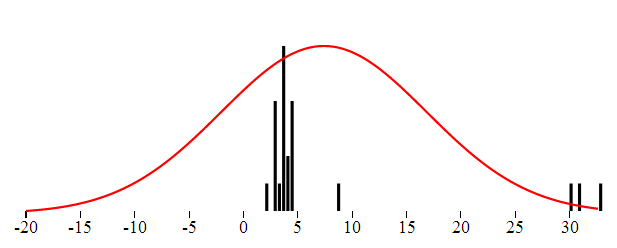
In perfect world the center is the mean value. That value is probably not a part of a data set but represents the typical value. The seconds measure which describes how far from the center the data is dispersed is called standard deviation. If we want to obtain the standard deviation from data we take the distance of each point from the center, square these values add them together and take square root. So we actually have all we need to get the distribution parameters from the data.

This approach of course has one main flaw. The mean value is affected by the outliers. And since the dispersion is deduced using the mean and outliers affect the mean value, the dispersion as well will be affected by them. In order to get a description of the dataset not affected by the extreme values one needs to find robust replacements for the mean and the dispersion.

Robust Center

The simplest and very efficient replacement for the mean as the center of the data is the median. Median is such value that half of the points in the dataset are smaller are bellow. That is if the data set consists of even number of samples, we just need to order the values and take mean of the two values in the middle of the ordered array. If the data consist of odd number of values then we take the element exactly in the middle of the ordered data. The before mentioned paper describes two more alternatives: trimmed mean, winsorized mean. Both of these are based on the exclusion of marginal values and I did not used them in my implementation.

Let's take the median of the given dataset and see if the distribution function based on it fits better the data. Even though the center is now in correct place the shape of the function does not fit completely the data from the histogram. That is because the variance is still affected by the outliers.

Robust Dispertion

Standard variance takes into account the the distance of all the numbers from the center. To rule out the extreme values, we can just use the median of distances. The outlier's distance from the center is much bigger than other distance and by taking the median of all distances we can get rid of outlier's influence over the dispersion. Here is the distribution function using this Robust type of dispersion. This characteristic is called MAD - Median Absolute Deviation.

Detecting the outliers

Now that we have the value of "real" center and "real spread" or dispersion we can state that the outlier is a value which differs "too much" from the center, taking into account the dispersion. Typically we could say that the outliers are such values that have a distance from center greater or equal to 10 * dispersion. The question is how to specify the multiplication coefficient. There is a statistics method called Hampel Indetifier which gives a formula to obtain the coefficient. Hampel identifier labels as outliers any points that are more than 5.2 away from the MAD. More details can be found here.

The overall reliability of this method

A question which might arise is up to which kind of messy data this method can be used. A common intuition would say that definitely more than the half of the data has to be "correct", in order to be able to detect the incorrect ones. To be able to measure the robustness of each method of detecting outliers, statisticians have introduced a term called Breakdown point. This point states which percentage of the data can be corrupted in order for given method to work. Using the Median as the center with the MAD (Median Absolute Deviation) has a breakdown point of 1/2. That is this method works if more than half of the data is correct. The standard arithmetic mean has a BP = 0. It is directly affected by all the numbers and one single outlier can completely move the data.

SQL implementation

In order to implement detection of outliers in SQL, one needs to first have the necessary functions to compute the mean, median and dispersion. All these functions are aggregates. Mean (avg) and Dispersion (var) are already implemented in SQL Server. If you are lucky enough to use SQL Server 2012 you can use the built-in median aggregate as well. The robust dispersion however has to be implemented manually even on SQL Server 2012.

Implementing aggregates for SQL Server is very easy, thanks to the predefined Visual Studio template. This templates will create a class for you which implements the IBinarySerializable interface and is decorate with couple attributes defined in the Microsoft.SqlServer namespace.

This class has 4 important methods:

• Init - anything needed before starting the aggregation
• Accumulate - adding one single value to the aggregate
• Merge - merging two aggregates
• Terminate - work to be done before returning the result of the aggregate

Here is the example of the Median aggregate

private List ld;

public void Init()
{
    ld = new List();
}

public void Accumulate(SqlDouble value)
{
    if (!value.IsNull)
    {
        ld.Add(value.Value);
    }
}

public void Merge(Median group)
{
    ld.AddRange(group.ld.ToArray());
}

public SqlDouble Terminate()
{
    return Tools.Median(ld);
}

Note that some aggregates can be computed iteratively. In that case all the necessary logic is in the Accumulate method and the Terminate method can be empty. With Median this is not the case (even though some iterative estimation methods exist. For the sake of the completeness, here is the implementation of median that I am using. It is the standard way: sorting the array and taking the middle element or average of the two middle elements. I am returning directly SqlDouble value, which is the result of the aggregate.

public static SqlDouble Median(List ld)
{
    if (ld.Count == 0)
        return SqlDouble.Null;

    ld.Sort();
    int index = ld.Count / 2;

    if (ld.Count % 2 == 0)
    {
        return (ld[index] + ld[index - 1]) / 2;
    }
    return ld[index];
}

Implementing the Robust variance using the MAD method is very similar, everything happens inside the Terminate method.

public SqlDouble Terminate()
{
    var distances = new List();
    var median = Tools.Median(ld);

    foreach (var item in ld)
    {
        var distance = Math.Abs(item - median.Value);
        distances.Add(distance);
    }

    var distMedian = Tools.Median(distances);
    return distMedian;
}

That implementation is directly the one described above: we take the distance of each element from the center (median) and than we take the median of the distances.

Outliers detection with the SQL aggregates

Having implemented both aggregates, detecting the outlier is just a matter of a SQL query - giving all the elements which are further away from the center than the variance multiplied by a coefficient.

select * from tbUsers where Height > ( Median(Height) + c*RobustVar(Height)) or Height < (Median(Height) - c*RobustVar(Height))

You will have to play with the coefficient value c to determine which multiplication gives you the best results.

JavaScript implementation

The same can be implemented in JavaScript. If you are interested in a JavaScript implementation you can check out the histogram chart from KoExtensions. This charting tool draws the histogram and the data distribution function. You can than configure it to use either Median or Mean as the center of the data as well as to use MAD, or standard variance to describe the dispersion.

KoExtensions is based on Knockout.JS and adds several useful bindings and the majority of them to simplify charting. Behind the scenes the data is charted using D3.

To draw a histogram chart with the distribution and detecting the outliers at the same time one needs just few lines of code

<div id="histogram" data-bind="histogram: data, chartOptions : {
        tolerance : 10,
        showProbabilityDistribution: true,min : -20,
        expected: 'median',
        useMAD: true,
        showOutliers: true}">

var exData = [3.9,3.8,3.9,2.7,2.8,1.9,2.7,3.5, 4.4, 2.8, 3.4, 8.6, 4.5, 3.5, 3.6, 3.8, 4.3, 4.5, 3.5,30,33,31];
  
function TestViewModel() {
    var self = this;
    self.data = ko.observableArray(exData);
}

var vm = new TestViewModel();
ko.applyBindings(vm);
initializeCharts();

Knockout.JS is a JavaScript MVVM framework tool which gives you all you need to create bi-directional binding between the view and the view model, where you can encapsulate and unit test all your logic. KoExtensions adds a binding call "histogram", which takes simple array and draws a histogram. In order to show the probability function and the outliers one has to set the options of the chart as shown in the example above.

Introduction to GPU programing through AMP C++

Few months ago I tried to learn a bit about GPU programming and I took notes a started to write this post. I am publishing this now even though it's not complete, however being too busy, I am not sure whether I will have the time to get back to this later.

Since couple years CUDA (*2007) and OpenCL (*2008) have established themselves as standard frameworks for parallel programming on the GPU. In 2011 new framework came to the landscape of GPGPU programming, which does not compete on the same level, but rather represents new abstraction between the GPU and the developer.

AMP stands for Accelerated Massive Parallelism and it is an open C++ standard. The implementation of AMP provided by Microsoft consists of three main features:

• C++ language features and compiler
• Runtime
• Programming framework containing classes and functions to facilitate parallel programming

As well as OpenCL and unlike CUDA, AMP is a standard not only for GPU programming but for any data-parallel hardware. Typical example of such a hardware is the vector unit of standard CPU, capable of executing SIMD (Single Instruction Multiple Data) instructions. Or in the near future a cloud based cluster. AMP is an abstraction layer which can be used to target different devices from different vendors.

The following diagram depicts how AMP C++ fits to the world of GPGPU programming.

Microsoft has implemented AMP on top of DirectCompute technology and it is the only production ready implementation. Currently there are also two Proof Of Concepts AMP implementations Shelvin park project done by Intel and open source modification of the LLVM compiler (more information here). Needless to say that the adoption of such standard will depend a lot on whether these implementations will be taken further and whether we will have real implementation based on CUDA.

First look at the code

Without further introduction let's take a look at the classical "Hello World" of GPGPU programming: Addition of elements of two vectors (here without the boiler plate code).

parallel_for_each(e,[=](index<2>idx) restrict(amp){
 c[idx] = a[idx] + b[idx];
});

If you have ever tried out OpenCL or CUDA, you should find this piece of code less verbose and quite easy to read. That is the result of the main ideas behind AMP C++:

• Full C++ - unlike CUDA or OpenCL, AMP is not a C like dialect.
• Minimalist API - AMP hides as much as it can from the developer.
• Future proofed - the API is designed for heterogeneous programming. In the future GPU should be only one of it's usages. It aims to be a standard for programming on distributed systems.

Before going futher with more examples we have to provide basic description of GPU architecture as it is crutial to understanding certain parts of AMP

GPU architecture

Here I will give a high level overview of the GPU architecture. If you are already familiar with the GPU architecture, feel free to skip this section.

Currently there are two main producers of GPU chips: NVidia and ATI (AMD). A little behind comes Intel. Each of them constructs graphic cards with different architecture. Moreover the architectures change significantly with the realease of any new version. Nevertheless certain concepts are shared by all of them. I will describe here shortly the NVidias Fermi and ATIs Cypress architecture. The succesor of Fermi is called Kepler.

Processor architecture

The GPU is composed of hundreds of pipelined cores. The cores are grouped to computation units. NVidia calls these units Symmetric Multiprocessors. Each computation unit is assigned a unit of work.

ATI uses slightly different abstraction. Similary to NVidia the "cores" are grouped to Symmetric Multiprocessors, however each core is called Thread Processor and is a capable of executing VLIV (Very Long Instruction Word) instructions. It has therefore 4 arithmetic logical units and one Special Function Unit. The compiler has to find independent operations and construct the VLIW instruction. If the compiler is not able to find these independent operations than one or more of the ALUs will not be performing any operation.

Memory access

The GPU has a global memory which can be accessed by all cores. This access is quite costly (hundreds of cycles). Each simetric multiprocessor in turn has a small scratch-pad memory which is called usually local memory. This memory can be accessed only by the threads running on the given SM. The access to local memory is much cheaper (around 10 cycles). This memory can either take a role of a cache or can be managed by the developer directly. In addition each core has its own general purpose registers, used to perform the computations.

GPUs usually run computations on data which is accessed only once, unlike CPUs where the same memory pages are often used repetively. For this reason it is better for the developer to control the local memory. That's why historically the local memory did not act as cache on GPUs. However this will probably change in the future, and some form of caching will be provided by the GPU directly.

Scheduling

Scheduling is essential because it allows the effective usage of the processor. Since the memory access is expensive, other operations might be executed while the processor is waiting for the data to come. NVidia processors have "costless" context switching, so while one thread is blocked other can take over. Therefore the number of threads scheduled might affect the computation performance, while if not enough threads are available for scheduling some might be waiting for the memory page loads.

The programming models comparison:

These architectural concepts are used by NVIDIA and ATI. Each of the 3 GPU programming models (CUDA, OpenCL, AMP) can has its own dialects and namings. The following table shows the terms used by all three technologies. We will discuss the AMP terms used in this table later in the article.

Term	CUDA	AMP C++	OpenCL
Basic unit of work	thread	thread	work-item
The code executed on one item	kernel	kernel	kernel
The unit processing one group of working units	Streaming multiprocessor	-	Compute unit
Cache-style memory accessible by grouped threads	shared memory	tile static memory	local memory
Group of working units sharing local memory	warp	tile	work-group

The tools offered by each framework

Now when the architecture of GPU has been described we can define the tools which each framework needs to provide. In the next part of the article I will try to describe how AMP adresses these issues.

• Tell the compiler which part of the code will be offloaded to the GPU
• Provide constructs to work with multidimensional vectors
• Provide a way to transfer the data between the GPU and the CPU
• Give the developer tools to write efficient programs. That is to address GPU specific problems such as memory access

AMP detailed description and more examples

Here is again the first example with the little of boiler plate code that we have to write to make it work:

void vectorsAddition_Parallel(vector<float> vA, vector<float> vB, vector<float>vC, int M, int N){
 extent<2> e(M,N);
 array_view<float,2> a(e, vA), b(e,vB);
 array_view<float,2> c(e, vC);


 //capture of the data using array_view -> results in the copy of the data into the accelerators memmory.
 parallel_for_each(e,[=](index<2>idx) restrict(amp){
  c[idx] = a[idx] + b[idx];
 });
}

The code sent and executed on the GPU is called "kernel" (here one line of code). The kernel is passed to the GPU in the form of lambda expression through the parallel_for_each method. This static method is the entry point to AMP. This method takes two parameters parallel_for_each(extent, delegate). The extend parameter describes the dimensionality of the data. The delegate encapsulates the logic which will be executed. The logic is usually defined as an anonymous function which takes the index<N> as parameter. The computation is expressed using this index on previously defined arrays. In the aboved sample the c[idx] = a[idx] + b[idx] simply means, that for each index (and index goes from 0,0 to N,N since it is two dimensional index) the elements at these positions of the arrays will be added and stored in the array c. Of course that this code is not executed sequentially, but instead defined as a set of vector operations which are scheduled on the GPU

The extent as well as the index parameter are templated. The index identifies one unique position in N dimensional array. The extent describes the dimensions of the computation domain.

The array_view class takes care of the copy of the data to and from the GPU. When the computation is finished, the synchronized method is called on the vC array_view. This call will synchronize the C vector with the array_view. To give the complete information, note also that there is an array class which behaves similary, having few inconvenience and advantages. This post gives a good comparison of these two classes.

The following example ilustrates some of the dificulties which we can have when writing parallel code. The code simply sums all the elements in an array in parallel way. The parallelization of addition of items requires a bit of engineering, even though the sequential solution is evident. Here I am using a technique which is not really efficient but demonstrates the principles of parallelization. Several techniques to parallelize the task are described in this article.

float sumArray_NaiveAMP(std::vector<float> items){
 auto size = items.size();
 array_view<float, 1> aV (size, items);
 
 for(int i=1;i<size;i=2*i){
  parallel_for_each(extent<1>(size/2), [=] (index<1> idx) restrict(amp)
  {
   aV[2*idx*i] = aV[2*idx*i] + aV[2*idx*i+i];
  });
 }

 return aV[0];
}

The algorihtm adds each two neighbouring items and stores the result in the first item. This has to be repeated until the addition of the whole array is stored in the first position in the array. As described in the mentioned article this approach is not memory efficient and optimizations exists. Note also that the synchronize method is not called on the array_view at the end of the computation. That is because, we don't want the modified data to be copied back from the GPU to the main memory, we are only interested in the sum of the elements.

Another example here is the computation of the standard deviation of the values in an array. First step is the computation of the avarage of the array. To obtain the avarege we have to first add the elements in the array (using the previous example). Having the average, we can obtain the distance of each element from the average. Once we have the distance of each element, we have to make another addition before taking the final square root and obtaining the standard deviation.

float standatd_deviation(vector<float> vA) {
 
 float size = vA.size();
 
 extent<1> e((int)size);
 vector<float> vDistance(size);
 
 array_view<float, 1> a(e, vA);
 array_view<float, 1> distance(e,vDistance);
 
 float dispertion = 0;
 float total = 0; 
 total = sumArray_NaiveAMP(vA);
 float avg = total/size;

 parallel_for_each(
  e, 
  [=](index<1> idx) restrict(amp) {
    distance[idx] = (a[idx] - avg)*(a[idx] - avg);

 });

 distance.synchronize();
 dispertion = sumArray_NaiveAMP(vDistance);
 return sqrt(dispertion/size);
}

This algorithm has 3 parallelized parts: the two sums at the beginning and at the end, and than the calculation of the distance of each element.

Looking at both of the preceding examples, you might be wondering why the code is so complex and you might think that the sum of the elements in the array could be just written as:

float sum = 0;
parallel_for_each(
 e, 
 [=](index<1> idx) restrict(amp) {
   sum+=a[idx];

});

However if you think a bit more, you should understand that the code in the parallel_for_each runs essential in the same time. All the parallel threads would like to increment the sum variable at the same time. In addition to that, this code would not even compile, while the modifications of variables captured "by value" are not allowed and in this example the sum variable is captured by value. If you are not familiar with the different capture types refer to this page.

Here is one more example which ilustrates how index and extent work, it is the second hello world of parallel computing: matrix multiplication. This example come from this MSDN page.

void matrixMultiplicationWithAMP(vector<float> &vC, vector<float> vA, vector<float> vB, int M, int N) {
 
 extent<2> e(M,N);

 array_view<float, 2> a(e, vA);
 array_view<float, 2> b(e,vB);
 array_view<float, 2> product(e, vC);
 

 parallel_for_each(
  product.extent, 
  [=](index<2> idx) restrict(amp) {
   int row = idx[0];
   int col = idx[1];
   for (int inner = 0; inner < M; inner++) {
    product[idx] += a(row,inner) * b(inner,col);
   }
 }
 );

 product.synchronize();
}

Note that the resulting vector vC i passed to the method as reference, since it's content is modified by the synchronize call. Also note, that this example assumes that the vectors passed to the function contain two dimensional array of size (N,N). Since AMP supports multidimensional indexes, AMP runs over all the columns and all the rows automatically, just by iterating over the two-dimensional index. The inner loop just sums the multiplications of the elements in the current row of the left matrix and the current column of the right matrix.

Moving the data between GPU and CPU

As mentioned before, the array_view and array classes are used to transfer the data between the CPU and GPU. The array class directly copies the data to the GPUs global memory. However the data from the array has to be then sent manually back to the CPUs memmory. On the other hand the array_view class works as a wrapper. The vector passed to the array_view will in the background copy the data from and to the vector which is passed in as parameter.

Memory access and manipulation on AMP

As described above, the developer has to address the GPU and adapt the algorithm to the architecture. This basically means minimize the access to global memmory and optimize the threads to use the local memmory. This process is called tiling in the AMP's parlance and the local memmory is called tile-static memory.

If the developer does not define any tiling, the code will be tiled by default. In order to use the local memory efficiently, algorithm has to be tiled manualy. Parallel_for_each method has a second overload which accepts tile_extent as a parameter and the code receives tiled_index in the lambda. Similary as the extend the tile_extend specifies the dimensionality of the computation domain, but also separates the whole computation domain into several tiles. Each tile is than treated by one symetrical multiprocessor, therefor all the threads in the tile can share the local memory and benefit from the fast memory access. If you want to read a bit more about tiling visit this page.

About the future of AMP

As said at the beginning AMP is a standard and as any standard it is dependent of it's implementations. Currently there are two existing implementations of the AMP standard. Microsoft implemented AMP on top of Direct Compute technology. Direct Compute is a part of Microsoft's DirectX suite, which was originally suited only to multimedia programming. Microsoft added DirectComputed to the DirectX suite in order to enable GPGPU programming and with AMP C++ provides an easy way to manipulate the API. The second implementation is very recent and was developed by Intel under the code name Shelvin Park. This implementation builds on top of OpenCL.

Summary

Clearly the success of the standard depends on whether other implementations targeting CUDA and OpenCL will emerge. Microsoft cooperated with NVidia and AMD during the development of the API. The idea of having a clear C++ standard to define the parallel computation is great. Latest C++ is quite modern language and provides nice constructs, so actually the programming using AMP C++ is quite fun and not that much pain.

Links

Introduction and few samples Parallel Programing in Native Code - blog of the AMP team

CUDA architecture evolution

GeForce GTX 680 Kepler Architecture

Comparison between CUDA and OpenCL (though little outdated 2011-06-22)

http://msdn.microsoft.com/en-us/library/hh553049.aspx

Introduction to Tiling

Implementation of LLVM & Clang to support AMP C++ on NVidia